Git log – Quick Reference

Some useful git log and git show options which I am bound to forget and will be happy to have in a singe place!

Limit the log entries

$ git log -<number of entries>
ex: git log -2 shows the last two commit details
$ git log -2
commit 474ea8e80dc30576b8b8f764a4f52c72e54277bd
Author: Nikhil Kuriakose <nikhilkuria@hotmail.com>
Date: Tue Sep 16 20:38:39 2014 +0530

draft v0.1 changes added

commit 3ac4e6fae7098951746dc46947bd12baec4b1f22
Author: nikhilkuria <nikhilkuria@hotmail.com>
Date: Fri Aug 29 09:55:53 2014 +0530

Bug fix : Some nodes were having trouble finding their parent.. phew!!

OK, so how about if we want to look at all the commits made since yesterday? All we need is the --since option:

git log --since="yesterday"

We can also use --until to fetch all commits up to a certain date; or of course we can use both options in tandem:

git log --since="1 week ago" --until="yesterday"

There is also a neat way to search the commits. Suppose you are working on a method and you need to know the history of changes made on it. Say, I am interested in the method, updateMetaDataMaps

git log -SupdateMetaDataMaps

This shows the commits that introduced a change to the code that added or removed that string.

Neat formats to the log

A simple git log statement gives us so much information that i need at the moment.

$ git log
commit 474ea8e80dc30576b8b8f764a4f52c72e54277bd
Author: Nikhil Kuriakose <nikhilkuria@hotmail.com>
Date: Tue Sep 16 20:38:39 2014 +0530

draft v0.1 changes added

commit 3ac4e6fae7098951746dc46947bd12baec4b1f22
Author: nikhilkuria <nikhilkuria@hotmail.com>
Date: Fri Aug 29 09:55:53 2014 +0530

Bug fix : Some nodes were having trouble finding their parent.. phew!!

commit 0051792ee0808e781a17d95cfb0d7b56a4402335
Author: = <=>
Date: Wed Aug 27 18:07:28 2014 +0530

Sensible to split the attributes

commit 1da57b8e21ace5238a6303920f52cf7363882067
Author: ueec6tv <extern_kuriakose.nikhil@allianz.com>
Date: Tue Aug 19 17:20:12 2014 +0530

extra lines!!!

And if you think you need even more information, the file changes can be shown using

$ git log -p

But, if you just need to see a minimal view, the –pretty=oneline option will help,

$ git log --pretty=oneline
474ea8e80dc30576b8b8f764a4f52c72e54277bd draft v0.1 changes added
3ac4e6fae7098951746dc46947bd12baec4b1f22 Bug fix : Some nodes were having trouble finding their parent.. phew!!
0051792ee0808e781a17d95cfb0d7b56a4402335 Sensible to split the attributes
1da57b8e21ace5238a6303920f52cf7363882067 extra lines!!!
eeb5c9a33462c2bfb6c058b55bbf6cb97d799607 Adding a sample xml file

–pretty also comes with options short, full and fuller options to show the output in roughly the same format but with less or more information, respectively

$ git log --pretty=short
commit 474ea8e80dc30576b8b8f764a4f52c72e54277bd
Author: Nikhil Kuriakose <nikhilkuria@hotmail.com>

draft v0.1 changes added

commit 3ac4e6fae7098951746dc46947bd12baec4b1f22
Author: nikhilkuria <nikhilkuria@hotmail.com>

Bug fix : Some nodes were having trouble finding their parent.. phew!!
$ git log --pretty=fuller
commit 474ea8e80dc30576b8b8f764a4f52c72e54277bd
Author: Nikhil Kuriakose <nikhilkuria@hotmail.com>
AuthorDate: Tue Sep 16 20:38:39 2014 +0530
Commit: Nikhil Kuriakose <nikhilkuria@hotmail.com>
CommitDate: Tue Sep 16 20:38:39 2014 +0530

draft v0.1 changes added

commit 3ac4e6fae7098951746dc46947bd12baec4b1f22
Author: nikhilkuria <nikhilkuria@hotmail.com>
AuthorDate: Fri Aug 29 09:55:53 2014 +0530
Commit: nikhilkuria <nikhilkuria@hotmail.com>
CommitDate: Fri Aug 29 09:55:53 2014 +0530

Bug fix : Some nodes were having trouble finding their parent.. phew!!

One of the most frequent things I have to do is find a commit based on a comment and see the changes. For example, I need to see the changes I made for a defect XYZ. I dont remember when I made the change, but I am sure, I will have the defect ID in the comment.

This is where the –pretty=oneline comes in handy, because the comment and the hash will be in one line

$ git log --pretty=oneline --grep="5716"
3546c34211dfa2de1477ee8a1c12d075ccc3729b fix for td 5716. adding extra validation

now, if i get the hash, i can quickly do a git show to see the changes i made,

$ git show 3546c34211dfa2de1477ee8a1c12d075ccc3729b

Bit shift operations – Quick Reference

Shifting the taking the binary equivalent of a number and moving the bit pattern left or right.

Left Shift Operator <<

Widely understood using the operator <<

Takes in two arguments – The sequence of binary values & number of shift operations

This operator shifts the first operand the specified number of bits to the left. Excess bits shifted off to the left are discarded. Zero bits are shifted in from the right.

  • Consider 12 whose binary equivalent is 00000000 00000000 00000000 00001100 (binary for 32 bits). Remember that the type operands (such as byte and short) are implicitly promoted to the int type before any shift operators are applied. Let’s shift it left 2 times.
    00000000 00000000 00000000 00001100 << 2(times)

    When you shift left ( << ) the void left behind by the shift is filled by zero’s. This is the result of (12<<2):

    00000000 00000000 00000000 00110000 (48)
  • Consider -12 whose binary equivalent is 11111111 11111111 11111111 11110100 (binary for 32 bits). Let’s shift it left 2 times.
    11111111 11111111 11111111 11110100 << 2(times)

    When you shift left ( << ) the void left behind by the shift is filled by zero’s. This is the result of (-12<<2):

    11111111 11111111 11111111 11010000 (-48)

    Let’s do -12<<28 and the result is

    01000000 00000000 00000000 00000000 (1073741824)

Right Shift Operator >>

Widely understood using the operator >>

Takes in two arguments – The sequence of binary values & number of shift operations

This operator shifts the first operand the specified number of bits to the right. Excess bits shifted off to the right are discarded. Copies of the leftmost bit are shifted in from the left.

  • Consider 12 whose binary equivalent is 00000000 00000000 00000000 00001100 (binary for 32 bits). Remember that the type operands (such as byte and short) are implicitly promoted to the int type before any shift operators are applied. Let’s shift it right 2 times.
    00000000 00000000 00000000 00001100 >> 2(times)

    When shifting right ( >> ) the leftmost bits exposed by the right shift are filled in with previous contents of the leftmost bit. This is the result of (12>>2):

    00000000 00000000 00000000 00000011 (3)
  • Consider -12 whose binary equivalent is 11111111 11111111 11111111 11110100 (binary for 32 bits). Let’s shift it right 2 times.
    11111111 11111111 11111111 11110100 >> 2(times)

    When shifting right ( >> ) the leftmost bits exposed by the right shift are filled in with previous contents of the leftmost bit. This is the result of (-12>>2):

    11111111 11111111 11111111 11111101 (-3)

Note that right shifting ( >> ) always preserves the sign of the original number i.e. to say that a negative number will stay negative while a positive number will stay positive after a right shift ( >> ).

Unsigned Right Shift Operator >>>

This operator shifts the first operand the specified number of bits to the right. Excess bits shifted off to the right are discarded. Zero bits are shifted in from the left.

When shifting right ( >> ) the leftmost bits exposed by the right shift are filled in with previous contents of the leftmost bit. BUT, the >>> unsigned right shift operator always fill zero’s and only zero’s no matter positive and negative number. For example,

  • Let’s do 00000000 00000000 00000000 00001100 >>> 2 (12>>>2) and the result is 00000000 00000000 00000000 00000011 (3).
  • Let’s do 11111111 11111111 11111111 11110100 >>> 2 (-12>>>2) and the result is 00111111 11111111 11111111 11111101 (1073741821).

Range of Shift Distance

If the promoted type of the left-hand operand is int, only the five lowest-order bits of the right-hand operand are used as the shift distance. It is as if the right-hand operand were subjected to a bitwise logical AND operator &  with the mask value 0x1f. The shift distance actually used is therefore always in the range 0 to 31, inclusive.

For example, the shift distance op2 is 34 in the op1 >> 34 (op1 is int type) . The 34’s binary equivalent is 00100010 and it over the rang [0,31]. The actually shift distance is op2 & 0x1f = 0x02. Thus, (op1 >> 34) has the same result as (op1 >> 2) .

Let’s take a look another example 12<<-3. The -3 binary representation is 11111101. Then op2= 0xfd & 0x1f = 0x1d = 29. The result of (12<<-3) has the same result as (12<<29).< /p>

If the promoted type of the left-hand operand is long, then only the six lowest-order bits of the right-hand operand are used as the shift distance. It is as if the right-hand operand were subjected to a bitwise logical AND operator &  with the mask value 0x3f. The shift distance actually used is therefore always in the range 0 to 63, inclusive.

For example, the shift distance op2 is 69 in the op1 >> 69 (op1 is long type) . The 69’s binary equivalent is 01000101 and it over the rang [0,63]. The actually shift distance is op2 & 0x3f = 0x05. Thus, (op1 >> 69) has the same result as (op1 >> 5) .

Application of Bit Shift Operations

Arithmetic

It can be seen from the example above that a Left shift of k position is same as multiplying the number with 2^k.

Similarly, a Right Shift of k position is same as multipying the number with 2^k.

Most compilers make use of this to optimize multiplication and division.

Random Number Generators

The elengant and efficient Random number algorithm by George Marsaglia uses Bit shift. Have a comprehensive read here.

Hash Generation Functions

There are quite many algorithms to generate Hash values which rely on Bit Shift operations. Good reference here.

How We Learned to Cheat at Online Poker: A Study in Software Security

by Brad Arkin, Frank Hill, Scott Marks, Matt Schmid and Thomas John Walls

Originally appeared on Developer.com; September 1999

Poker is a card game that many people around the world enjoy. Poker is played at kitchen tables, in casinos, and cardrooms — and more recently, the Web. A few of us here at Reliable Software Technologies play poker. Since many of us spend a good amount of our days online, it was only a matter of time before some of us put the two interests together. This is the story of how our interest in online poker and software security mixed to create a spectacular security exploit.

The PlanetPoker Internet cardroom offers real-time Texas Hold’em games against other people on the Web for real money. Being software professionals who help companies deliver secure, reliable, and robust software, we were curious about the software behind the online game. How did it work? Was it fair? An examination of the FAQs at PlanetPoker, including the shuffling algorithm (which was ironically published to help demonstrate the game’s integrity) was enough to start our analysis wheels rolling. As soon as we saw the shuffling algorithm, we began to suspect there might be a problem. A little investigation proved that this intuition was correct.

The Game

In Texas Hold’em, each player is dealt two cards (called the pocket cards). The initial deal is followed by a round of betting. After the first round, all remaining cards are dealt face up and shared by all players. The dealer places three cards face up on the board (called the flop). A second round of betting then takes place. Texas Hold’em is usually a fixed limit game, meaning that there are fixed amounts that a player may bet in each betting round. For example, in a $3 to $6 game, the first two betting rounds are $3 bets while the third and fourth betting rounds are $6 bets. After the second round of betting, the dealer places another card face up on the board (called the turn). A third round of betting then takes place. Finally, the dealer places the last card face up on the board (called the river), and a final round of betting ensues. Each remaining player takes their two pocket cards and combines them with the five community cards to make the best five-card poker hand. The best hand among the players is determined by standard poker hand order.

Texas Hold’em is a fast-paced and exciting game. Bluffing is an essential part of the game, and quick decisions about who is holding what sorts of cards separate winners from losers. Interestingly, Texas Hold’em is the poker game played at the World Series of Poker which is held annually in Las Vegas.

Now that everybody and their dog is online, and virtually all types of businesses are represented on the Internet, it’s only natural that casinos and cardrooms are there too. Even with the reasonably easy availability of casinos on Indian reservations and riverboats, there is still real demand for more accessible games. Being able to play online in the comfort of your own home (not to mention in your pajamas), without having to endure second-hand smoke and obnoxious players, is definitely appealing.

Security Risks Abound

All this convenience comes at a price. Unfortunately, there are real risks to playing poker online. The casino may be a fraud, existing only to take money from naïve players without ever intending to pay back winnings. The server running the online casino could be cracked by a malicious attacker looking for credit card numbers, or trying to leverage some advantage in the game. Since a majority of casinos don’t authenticate or encrypt the network traffic between the player running the client program and the server hosting the card game, a malicious player could conceivably examine the network traffic (with a classic person-in-the-middle attack) for the purposes of determining his opponent’s cards. These risks are all very familiar to Internet security experts.

Collusion is a problem that is unique to poker (as opposed to other games like blackjack or craps), since poker players play against each other and not the casino itself. Collusion occurs when two or more players seated at the same table work together as a team, often using the same bankroll. Colluding players know what their team members’ hands are (often through subtle signals), and bet with the purpose of maximizing their team’s profits on any given hand. Though collusion is a problem in real cardrooms, it is a much more serious problem for online poker. Using tools like instant messaging and telephone conference calls makes collusion a serious risk to online poker players. What if all the players in an online game are all cooperating to bilk an unsuspecting Web patsy? How can you be assured that you’re never a victim of this attack?

Last, but not least (especially in terms of our story), there is a real risk that the software behind an online poker game may be flawed. Software problems are a notorious form of security risk often overlooked by companies obsessed with firewalls and cryptography. The problem is that a software application can introduce truck-sized security holes into a system. We spend a great deal of time in our day jobs finding and solving software security problems. It is only natural that we turned our attention to online poker. The rest of this article is devoted to a discussion of software security problems we found in a popular online poker game.

Software Security Risks

Shuffling a Virtual Deck of Cards

The first software flaw we’ll focus on involves shuffling virtual cards. What does it mean to shuffle a deck of cards fairly? Essentially, every possible combination of cards should have an equal likelihood of appearing. We’ll call each such ordering of the 52 cards a shuffle.

In a real deck of cards, there are 52! (approximately 2^226) possible unique shuffles. When a computer shuffles a virtual deck of cards, it selects one of these possible combinations. There are many algorithms that can be used to shuffle a deck of cards, some of which are better than others (and some of which are just plain wrong).

We found that the algorithm used by ASF Software, Inc., the company that produces the software used by most of the online poker games, suffered from many flaws. ASF has changed their algorithm since we contacted them regarding our discovery. We have not looked at their new approach. Getting everything exactly right from a security perspective is not easy (as the rest of this article will show).

Figure 1: The Flawed ASF Shuffling Algorithm

procedure TDeck.Shuffle;
var
    ctr: Byte;
    tmp: Byte;

    random_number: Byte;
begin
    { Fill the deck with unique cards }
    for ctr := 1 to 52 do
        Card[ctr] := ctr;

    { Generate a new seed based on the system clock }
    randomize;

    { Randomly rearrange each card }
    for ctr := 1 to 52 do begin
        random_number := random(51)+1;
        tmp := card[random_number];
        card[random_number] := card[ctr];
        card[ctr] := tmp;
    end;

    CurrentCard := 1;
    JustShuffled := True;
end;

The shuffling algorithm shown in Figure 1 was posted by ASF Software in order to convince people that their computer-generated shuffles were entirely fair. Ironically, it had the exact opposite effect on us.

The algorithm starts by initializing an array with values in order from 1 to 52, representing the 52 possible cards. Then, the program initializes a pseudo-random number generator using the system clock with a call to Randomize(). The actual shuffle is performed by swapping every position in the array, in turn, with a randomly chosen position. The position to swap with is chosen by calls to the pseudo-random number generator.

Problem One: An Off-By-One Error

Astute programmers will have noticed that the algorithm in question contains an off-by-one error. The algorithm is supposed to traverse the initial deck while swapping each card with any other card. Unlike most Pascal functions, the function Random(n) actually returns a number between 0 and n-1 instead of a number between 1 and n. The algorithm uses the following snippet of code to choose which card to swap with the current card: . The formula sets random_number to a value between 1 and 51. In short, the algorithm in question never chooses to swap the current card with the last card. When ctr finally reaches the last card, 52, that card is swapped with any other card except itself. That means this shuffling algorithm never allows the 52nd card to end up in the 52nd place. This is an obvious, but easily correctable, violation of fairness.

Problem Two: Bad Distribution Of Shuffles

A closer examination of the shuffling algorithm reveals that, regardless of the off-by-one problem, it doesn’t return an even distribution of decks. The basic algorithm at the heart of the shuffle is shown in Figure 2.

Shuffling

A closer examination of the algorithm reveals that, regardless of the off-by-one error, it doesn’t return an even distribution of shuffles. That is, some shuffles are more likely to be produced than others are. This uneven distribution can be leveraged into an advantage if a tipped-off player is willing to sit at the table long enough.

To illustrate this problem using a small example, we’ll shuffle a deck consisting of only three cards (i.e, n=3) using the algorithm described above.

Figure 2: How not to shuffle cards

for (i is 1 to n)
    Swap i with random position between 1 and n
Figure 2

Figure 2 contains the algorithm we used to shuffle our deck of three cards, and also depicts the tree of all possible decks using this shuffling algorithm. If our random number source is a good one, then each leaf on the tree in Figure 2 has an equal probability of being produced.

Given even this small example, you can see that the algorithm does not produce shuffles with equal probability. It will produce the decks 231, 213, and 132 more often than the decks 312, 321, 123. If you were betting on the first card and you knew about these probabilities, you would know that card 2 is more likely to appear than any other card. The uneven probabilities become increasingly exaggerated as the number of cards in the deck increase. When a full deck of 52 cards is shuffled using the algorithm listed above (n=52), the unequal distribution of decks skews the probabilities of certain hands and changes the betting odds. Experienced poker players (who play the odds as a normal course of business) can take advantage of the skewed probabilities.

Figure 3: How to shuffle cards

for (i is 1 to 3)
    Swap i with random position between i and 3
Figure 3

Figure 3 provides a much better shuffling algorithm. The crucial difference between the two algorithms is that number of possible swap positions decreases as you progress through the deck. Once again, we show a tree illustrating this algorithm on our sample deck of three cards. The change between this new algorithm and the one used by ASF is that each card i is swapped with a card from the range [i, n], not [1, n]. This reduces the number of leaves from the 3^3 = 27 given by the bad algorithm listed above to 3! = 6. The change is important because the n! number of unique leaves means that the new shuffling algorithm generates each possible deck only once. Notice that each possible shuffle is produced once and only once so that each deck has an equal probability of occurring. Now that’s fair!

Generating Random Numbers on a Deterministic Machine

The first set of software flaws we discussed merely changes the probabilities that certain cards will come up. The associated skews can be used by a clever gambler to gain an edge, but the flaws really don’t constitute a complete break in the system. By contrast, the third flaw, which we explain in this section, is a doozy that allows online poker to be completely compromised. A short tutorial on pseudo-random number generators sets the stage for the rest of our story.

How Pseudo-Random Number Generators Work

Suppose we want to generate a random number between 1 and 52, where every number has an equal probability of appearing. Ideally, we would generate a value on the range from 0 to 1 where every value will occur with equal probability, regardless of the previous value, then multiply that value by 52. Note that there are an infinite number of values between 0 and 1. Also note that computers do not offer infinite precision!

In order to program a computer to do something like the algorithm presented above, a pseudo-random number generator typically produces an integer on the range from 0 to N and returns that number divided by N. The resulting number is always between 0 and 1. Subsequent calls to the generator take the integer result from the first run and pass it through a function to produce a new integer between 0 and N, then return the new integer divided by N. This means the number of unique values returned by any pseudo-random number generator is limited by number of integers between 0 and N. In most common random number generators, N is 2^32 (approximately 4 billion) which is the largest value that will fit into a 32-bit number. Put another way, there are at most 4 billion possible values produced by this sort of number generator. To tip our hand a bit, this 4 billion number is not all that large.

A number known as the seed is provided to a pseudo-random generator as an initial integer to pass through the function. The seed is used to get the ball rolling. Notice that there is nothing unpredictable about the output of a pseudo-random generator. Each value returned by a pseudo-random number generator is completely determined by the previous value it returned (and ultimately, the seed that started it all). If we know the integer used to compute any one value then we know every subsequent value returned from the generator.

The pseudo-random number generator distributed with Borland compilers makes a good example and is reproduced in Figure 4. If we know that the current value of RandSeed is 12345, then the next integer produced will be 1655067934 and the value returned will be 20. The same thing happens every time (which should not be surprising to anyone since computers are completely deterministic).

Figure 4: Borland’s implementation of Random()

long long RandSeed = #### ;

unsigned long Random(long max)
{
 long long x ;
 double i ;
 unsigned long final ;
 x = 0xffffffff;
 x += 1 ;

 RandSeed *= ((long long)134775813);
 RandSeed += 1 ;
 RandSeed = RandSeed % x ;
 i = ((double)RandSeed) / (double)0xffffffff ;
 final = (long) (max * i) ;

 return (unsigned long)final;
}

Based on historical precedent, seeds for number generators are usually produced based on the system clock. The idea is to use some aspect of system time as the seed. This implies if you can figure out what time a generator is seeded, you will know every value produced by the generator (including what order numbers will appear in). The upshot of all this is that there is nothing unpredictable about pseudo-random numbers. Needless to say, this fact has a profound impact on shuffling algorithms!

On To Poker, Or How To Use A Random Number Generator Badly

The shuffling algorithm used in the ASF software always starts with an ordered deck of cards, and then generates a sequence of random numbers used to re-order the deck. Recall that in a real deck of cards, there are 52! (approximately 2^226) possible unique shuffles. Also recall that the seed for a 32-bit random number generator must be a 32-bit number, meaning that there are just over 4 billion possible seeds. Since the deck is reinitialized and the generator re-seeded before each shuffle, only 4 billion possible shuffles can result from this algorithm. Four billion possible shuffles is alarmingly less than 52!.

To make matters worse, the algorithm of Figure 1 chooses the seed for the random number generator using the Pascal function Randomize(). This particular Randomize() function chooses a seed based on the number of milliseconds since midnight. There are a mere 86,400,000 milliseconds in a day. Since this number was being used as the seed for the random number generator, the number of possible decks now reduces to 86,400,000. Eight-six million is alarmingly less than four billion. But that’s not all. It gets worse.

Breaking the System

The system clock seed gave us an idea that reduced the number of possible shuffles even further. By synchronizing our program with the system clock on the server generating the pseudo-random number, we are able to reduce the number of possible combinations down to a number on the order of 200,000 possibilities. After that move, the system is ours, since searching through this tiny set of shuffles is trivial and can be done on a PC in real time.

The RST exploit itself requires five cards from the deck to be known. Based on the five known cards, our program searches through the few hundred thousand possible shuffles and deduces which one is a perfect match. In the case of Texas Hold’em poker, this means our program takes as input the two cards that the cheating player is dealt, plus the first three community cards that are dealt face up (the flop). These five cards are known after the first of four rounds of betting and are enough for us to determine (in real time, during play) the exact shuffle. Figure 5 shows the GUI we slapped on our exploit. The “Site Parameters” box in the upper left is used to synchronize the clocks. The “Game Parameters” box in the upper right is used to enter the five cards and initiate the search. Figure 5 is a screen shot taken after all cards have been determined by our program. We know who holds what cards, what the rest of the flop looks, and who is going to win in advance.

Figure 5: The GUI for our exploit

Figure 5

Once it knows the five cards, our program generates shuffles until it discovers the shuffle that contains the five cards in the proper order. Since the Randomize() function is based on the server’s system time, it is not very difficult to guess a starting seed with a reasonable degree of accuracy. (The closer you get, the fewer possible shuffles you have to look through.) Here’s the kicker though; after finding a correct seed once, it is possible to synchronize our exploit program with the server to within a few seconds. This post facto synchronization allows our program to determine the seed being used by the random number generator, and to identify the shuffle being used during all future games in less than one second!

Technical detail aside, our exploit garnered spectacular press coverage. The coverage emphasizes the human side of our discovery. See our Web site for our original press release, the CNN video clip, and a New York Times story.

Doing Things Properly, or How to Shuffle Virtual Cards

As we have shown, shuffling virtual cards isn’t as easy as it may appear at first blush. The best way to go about creating a shuffling algorithm is to develop a technique that can securely produce a well-shuffled deck of cards by relying on sound mathematics. Furthermore, we believe that publishing a good algorithm and opening it up to real-world scrutiny is a good idea (which meshes nicely with the opinions of the Open Source zealots). The main thing here is not relying on security by obscurity. Publishing a bad algorithm (like AFS did) is a bad idea, but so is not publishing a bad algorithm!

Cryptography relies on solid mathematics, not obscurity, to develop strong algorithms used to protect individual, government, and commercial secrets. We think shuffling is similar. We can stretch the analogy to include a parallel between cryptographic key length (which is directly proportional to the strength of many cryptographic algorithms) and the size of the random seed that is used to produce a shuffled deck of cards.

Developing a card-shuffling algorithm is a fairly straightforward task. The first thing to realize is that an algorithm capable of producing each of the 52! shuffles is not really required. The reasoning underlying this claim is that only an infinitesimally small percent of the 52! shuffles will ever be used during play. It is important, however, that the shuffles the algorithm produces maintain an even distribution of cards. A good distribution ensures that each position in the shuffle has an approximately equal chance of holding any one particular card. The distribution requirement is relatively easy to achieve and verify. The following pseudo-code gives a simple card-shuffling algorithm that, when paired with the right random number generator, produces decks of cards with an even distribution.

START WITH FRESH DECK
GET RANDOM SEED
FOR CT = 1, WHILE CT <= 52, DO
X = RANDOM NUMBER BETWEEN CT AND 52 INCLUSIVE
SWAP DECK[CT] WITH DECK[X]

Key to the success of our algorithm is the choice of a random number generator (RNG). The RNG has a direct impact on whether the algorithm above will successfully produce decks of even distribution as well as whether these decks will be useful for secure online card play. To begin with, the RNG itself must produce an even distribution of random numbers. Pseudo-random number generators (PRNG), such as those based on the Lehmer algorithm, have been shown to possess this mathematical property. It is therefore sufficient to use a good PRNG to produce “random” numbers for card shuffling.

As we have seen, choice of initial seed for the PRNG is a make or break proposition. Everything boils down to the seed. It’s absolutely essential that players using a deck of cards generated using a PRNG can’t determine the seed used to produce that particular shuffle.

A brute force attempt to determine the seed used to produce a particular shuffle can be made by systematically going through each of the possible seeds, producing the associated shuffle, and comparing the result against the deck you’re searching for. To avoid susceptibility to this kind of attack, the number of possible seeds needs to be large enough that it is computationally infeasible to perform an exhaustive search within certain time constraints. Note that on average only half of the seed space will need to be searched until a match is found. For the purposes of an online card game, the time constraint would be the length of that game, which is usually on the order of minutes.

In our experience, a simple program running on a Pentium 400 computer is able to examine approximately 2 million seeds per minute. At this rate, this single machine could exhaustively search a 32-bit seed space (2^32 possible seeds) in a little over a day. Although that time period is certainly beyond the time constraints we have imposed on ourselves, it is certainly not infeasible to use a network of computers to perform a distributed search within our real time bounds.

The subject of brute force attacks serves to emphasize the aptness of our analogy between key length in a cryptographic algorithm and the seed behind shuffling. A brute-force cryptographic attack involves attempting every possible key in order to decrypt a secret message. Likewise a brute-force attack against a shuffling algorithm involves examining every possible seed. A significant body of research studying the necessary lengths of cryptographic keys already exists. Generally speaking, things look like this:

Algorithm Weak Key Typical Key Strong Key
DES 40 or 56 56 Triple-DES
RC4 60 80 128
RSA 512 768 or 1024 2048
ECC 125 170 230

People used to think that cracking 56-bit DES in real time would take too long to be feasible, but history has shown otherwise. In January 1997, a secret DES key was recovered in 96 days. Later efforts broke keys in 41 days, then 56 hours, and, in January 1999, in 22 hours and 15 minutes. The leap forward in cracking ability doesn’t bode well for small key lengths or small sets of seeds!

People have even gone so far as to invent special machines to crack cryptographic algorithms. In 1998, the EFF created a special-purpose machine to crack DES messages. The purpose of the machine was to emphasize just how vulnerable DES (a popular, government-sanction algorithm) really is. (For more on the DES cracker, see http://www.eff.org/descracker/.) The ease of “breaking” DES is directly related to the length of its key. Special machines to uncover RNG seeds are not outside the realm of possibility.

We believe that a 32-bit seed space is not sufficient to resist a determined brute-force attack. On the other hand, a 64-bit seed should be resistant to almost any brute force attack. A 64-bit seed makes sense since many computers provide the ability to work with 64-bit integers off the shelf, and a 64-bit number should be sufficient for the purposes of protecting card shuffling against brute-force attacks.

64-bits alone won’t do it though. We can’t overemphasize that there must be absolutely no way for an attacker to predict or approximate the seed that is used by the PRNG. If there is a way to predict the seed, then the computationally-taxing brute-force attack outlined above becomes irrelevant (since the entire system breaks much more easily). In terms of our exploit, not only did ASF’s flawed approach rely on a too-small 32-bit PRNG, but the approach relies on a seed based on the time of day as well. As our exploit demonstrated, there is very little randomness in such an approach.

In final analysis, the security of the entire system relies on picking a random seed in a non-predictable manner. The best techniques for choosing such a random number are hardware-based. Hardware-based approaches rely on unpredictably random data gathered directly from the physical environment. Since online poker and other games involving real money are extremely security critical undertakings, it’s probably worth investing the necessary resources to ensure that random number generation is done correctly.

In concert, a good shuffling algorithm and a 64-bit pseudo-random number generator seeded with a proven hardware device should produce shuffles that are both fair and secure. Implementing a fair system is not overly difficult. Online poker players should demand it.

Borrowed from here.. too good I had to share..

RegEx to match Java Comments

Most(if not all) of the regular expressions a developer needs is already available. There are numerous resources online ranging from blogs and even an ever growing library. Not to mention the endless discussions on stackoverflow.

Few days back, I had lost the sources to a project and had to decompile them from the original build. Did not expect the decompiler to throw in so much comments.

Capture

The most obivious way to remove comments would be to use the following regEx.

/\*.*\*/

This seems the natural way to do it. /\* finds the start of the comment (note that the literal * needs to be escaped because * has a special meaning in regular expressions), .* finds any number of any character, and \*/ finds the end of the expression.

This will remove all the comments the decompiler put it. But, wanted to pursue more to handle any kind of comments.

The first problem with this approach is that .* does not match new lines. (Note, the text in green color is matched)

/* First comment 
 first comment—line two*/
/* Second comment */

This can be overcome easily by replacing the . with (.|[\r\n]):(\r and \n represent the return and newline characters)

/\*(.|[\r\n])*\*/

This reveals a second, more serious, problem—the expression matches too much. Regular expressions are greedy, they take in as much as they can. Consider the case in which your file has two comments. This regular expression will match them both along with anything in between:

start_code();
/* First comment */
more_code(); 
/* Second comment */
end_code();

To fix this, the regular expression must accept less. We cannot accept just any character with a ., we need to limit the types of characters that can be in our expressions. The new RegEx stops parsing when it sees a */ and will begin the next match only when it sees another /*.

/\*([^*]|[\r\n])*\*/

The disadvantage is that this simplistic approach doesn’t accept any comments with a * in them, which a standard java comment.

/* 
* Common multi-line comment style. 
*/ 
/* Second comment */

This is where it gets tricky. How do we accept a * without accepting the * that is part of the end comment? The solution is to still accept any character that is not *, but also accept a * and anything that follows it provided that it isn’t followed by a /. The parse will only stop if it sees a */ and will continue when it sees a *.

/\*([^*]|[\r\n]|(\*([^/]|[\r\n])))*\*/

Also, the section in bold makes sure * comes only in pairs. It will accept any even number of *. It might even accept the * that is supposed to end the comment.

start_code();
/****
 * Common multi-line comment style.
 ****/
more_code(); 
/*
 * Another common multi-line comment style.
 */
end_code();

We should also make sure that the comment can end in multiple * s.

/\*([^*]|[\r\n]|(\*+([^*/]|[\r\n])))*\*+/

This RegEx can be used to find/replace java comments using a standard text editor.

An easier Method

Most regular expression packages support non-greedy matching. This means that the pattern will only be matched if there is no other choice. We can modify our second try to use the non-greedy matcher *? instead of the greedy matcher *. With this change, the middle of our comment will only match if it doesn’t match the end:

/\*(.|[\r\n])*?\*/

On the beauty of Algorithms.. Part 1

As software engineers, our job is not just to find solution to problems, but to find the best solution to a problem.

You don’t aspire to be just another monkey with a fancy title..

Monkey-typing

Had the chance to comeupon a few beautifully crafted courses online. Highly reccomend to checkout this, this and this..

To demonstate the power of a good algorithms, let’s borrow a case study from Sedgewick and Wayne’s beautifully crafted book.

The Dynamic Connectivity problem 

We start with the following problem specification: The input is a sequence of pairs of integers, where each integer represents an object of some type and we are to interpret the pair p q as meaning “p is connected to q.”

We assume that “is connected to” is an equivalence relation, which means that it is
■ Reflexive : p is connected to p.
■ Symmetric : If p is connected to q, then q is connected to p.
■ Transitive : If p is connected to q and q is connected to r, then p is connected to r.

An equivalence relation partitions the objects into equivalence classes. In this case, two objects are in the same equivalence class if and only if they are connected. Our goal is to write a program to filter out extraneous pairs (pairs where both objects are in the same equivalence class) from the sequence.

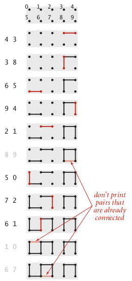
See the illustration below,

union find

Assume the universe consists of 10 points numbered from 0-9. Initially none of the points are connected. The inputs are the pair of numbers on the left.

The first pair (4,3). We check if there exists a connection between the pair. So, we create  a connection between the two nodes and prints out the connection. Same for the next 4 inputs of (3,8), (6,5), (9,4) and (2,1).

But the next input, (8,9). Even though there is no direct connection between 8 and 9, they are part of a connected component, [3,4,8,9]. So, no new connection is to be made and nothing is printed. And so on..

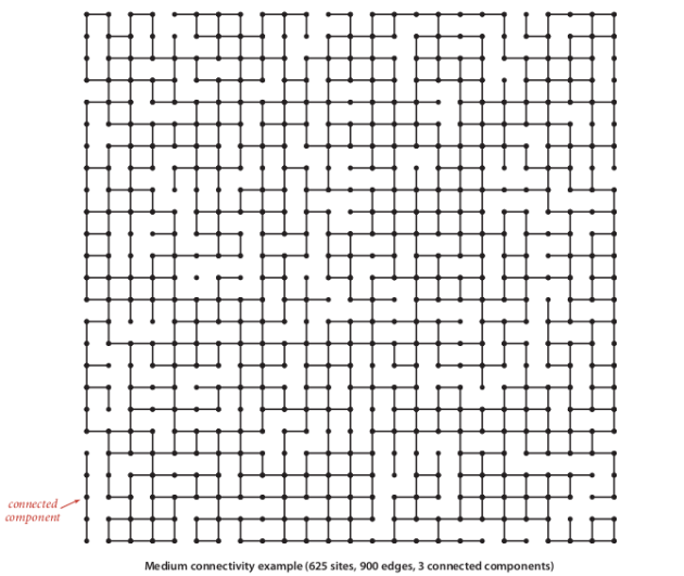
Given a grid with numerous connected components, identifying the connected components or if two nodes are connected pose a computational problem. See the universe below,

union find2

You can quickly identify component consisting of five sites at the bottom left, but you might have difficulty verifying that all of the other sites are connected to one another. For a program, the task is
even more difficult, because it has to work just with site names and connections and has no access to the geometric placement of sites in the diagram. How can we tell quickly whether or not any given two sites in such a network are connected?

A solution to the problem provides an effective implementation for,

void union(int p, int q) – add connection between p and q
int find(int p) – component identifier for p (0 to N-1)
boolean connected(int p, int q) – return true if p and q are in the same component

The union() operation merges two components if the two sites are in different components, the find() operation returns an integer component identifier for a given site, the connected() operation determines whether two sites are in the same component.

As we shall soon see, the development of an algorithmic solution for dynamic connectivity thus reduces to the task of developing an implementation of this API. Every implementation has to
■ Define a data structure to represent the known connections
■ Develop efficient union(), find(), connected() implementations that are based on that data structure

As usual, the nature of the data structure has a direct impact on the efficiency of the algorithms, so data structure and algorithm design go hand in hand. The API already specifies the convention that both sites and components will be identified by int values between 0 and N-1, so it makes sense to use a site-indexed array id[] as our basic data structure to represent the components.

Initially, none of the sites are connected and each site corresponds to a component. Initially, we start with N components, each site in its own component, so we initialize id[i] to i for all i from 0 to N-1.

All of our implementa-tions use a one-line implementation of connected() that returns the boolean value find(p) == find(q). The find(int p) methods returns the identified for the component. So, it should make perfect sense to assert that, if two sites correspond to the same component, they are connected.

Implementations 

We shall consider three different implementations, all based on using the site-indexed id[] array, to determine whether two sites are in the same connected component.

Quick-find

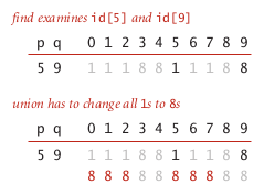
One approach is to maintain the invariant that p and q are connected if and only if id[p] is equal to id[q]. In other words, all sites in a component must have the same value in id[]. This method is called quick-find because find(p) just returns id[p], which immediately implies that connected(p, q) reduces to just the test id[p] == id[q] and returns true if and only if p and q are in the same component.

For implementing union, we first check whether they are already in the same component, in which case there is nothing to do. Otherwise, we are faced with the situation that all of the id[] entries corresponding to sites in the same component as p have one value and all of the id[] entries corresponding to sites in the same component as q have another value. To combine the two components into one, we have to make all of the id[] entries corresponding to both sets of sites the same value, as shown in the example. To do so, we go through the array, changing all the entries with values equal to id[p] to the value id[q].

We could have decided to change all the entries equal to id[q] to the value id[p]—the choice between these two alternatives is arbitrary.

union find3

The implementation is pretty simple,

public int find(int p)
{ return id[p]; }
public void union(int p, int q)
{  // Put p and q into the same component.
   int pID = find(p);
   int qID = find(q);
   // Nothing to do if p and q are already in the same component.
   if (pID == qID) return;
      // Rename p’s component to q’s name.
      for (int i = 0; i < id.length; i++){
         if (id[i] == pID) {
           id[i] = qID;
         }
         count--;
      }
}

The find() operation is certainly quick, as it only accesses the id[] array once in order to complete the operation. But quick-find is typically not useful for large problems because union() needs to scan through the whole id[] array for each input pair.

In particular, suppose that we use quick-find for the dynamic connectivity problem and wind up with a single component. This requires at least (N-1) calls to union(). union() iterates through all the n elements at least once, which clearly gives us a N 2 complexity. This analysis generalizes to say that quick-find is quadratic for typical applications where we end up with a small number of components. Modern computers can execute hundreds of millions or billions of instructions per second, so this cost is not noticeable if N is small, but we also might find ourselves with millions or billions of sites and connections to process in a modern application. Trying to solve a problem with millions or billions of sites will not give us an acceptable time.

Most defenitely Quick-Find can be impoved..


Navigating XML Graph using Cypher

Cypher is a neat way to manipulate a Neo4j database. It would be equally amazing if the Xml graph could be queried with Cypher as well.

Honestly, I must put credits to Michael for suggesting such a possibility here..

Well, let’s start with a simple xml file.

<library>
<author firstname="Earnest" lastname="Hemingway">
<works>
<book name="A Farewell to Arms" year="1929" />
<book name="For Whom the bell tolls" year="1940" />
<book name="The Old man and the sea" year="1951" />
</works>
<awards>
<award name = "Pulitzer Prize" category="Fiction" year="1953"></award>
<award name = "Nobel Prize" category="Literature" year="1954"></award>
</awards>
</author>
<author firstname="Victor" lastname="Hugo">
<works>
<book name="The Hunchback of Notre-Dame" year="1831" />
<book name="Les Misérables" year="1862" />
</works>
</author>
</library>

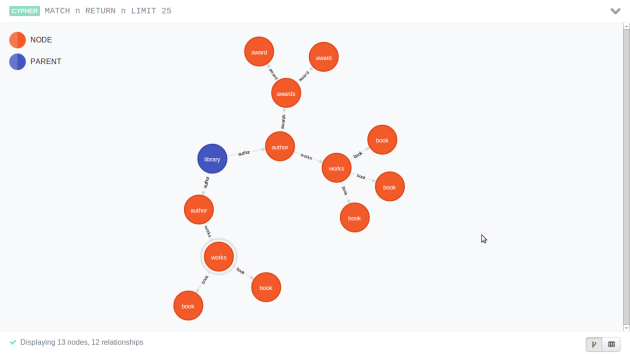
It’s a simple xml with nothing fancy in it. As explained in the previous posts here and here.. A neat neo4j graph can be made out of this…

Screenshot from 2014-07-22 21:16:46

So, let’s go about traversing this graph using Cypher.. And since we are trying to traverse an XML, let’s make a rough comparison to XPath.

Let’s fetch all the book nodes,

The Xpath to get all the book nodes, no matter where they are in the document, is

//book

For the same purpose, the Cypher query would be,

MATCH (books:book) RETURN books

This will fetch the following output for the above Graph,


bookNodes


Let’s now try to fetch the name of all books. The XPath will require only a slight modification,

//book/@name

The XPath will return the list as,

Attribute='name="A Farewell to Arms"'
Attribute='name="For Whom the bell tolls"'
Attribute='name="The Old man and the sea"'
Attribute='name="The Hunchback of Notre-Dame"'
Attribute='name="Les Misérables"'

The Cypher will only require a small modification. Instead of returning the entire node, fetch the ‘name’ attribute for the nodes.

MATCH (books:book) RETURN books.name

bookName Next up, let’s query the awards honoured to Earnest Hemingway,

This can be achieved via XPath as,

//author[@firstname=’Earnest’]/awards

which gives the output

<awards>
  <award name="Pulitzer Prize" category="Fiction" year="1953" />
  <award name="Nobel Prize" category="Literature" year="1954" />
</awards>

As for Cypher,

MATCH (author {firstname: “Earnest”})-[*]->(award:award) RETURN award

We try to fetch any node of the type ‘award’ connected to a node of type ‘author’ with firstname = Earnest

awards

The above examples are very much trivial, and aims to prove the possibility of using Cypher to traverse a database. I am looking for a huge and most importantly meaningful xml content which can be queried to get some useful information. Keep watching this space for more..

Implementing Word Ladder game using Neo4j

Word Ladder is a pretty popular game invented by Lewis Carroll, who is better known as the author of Alice in Wonderland.

In a word ladder puzzle you must make the change occur gradually by changing one letter at a time. At each step you must transform one word into another word, you are not allowed to transform a word into a non-word. For instance, the word “FOOL” can be transformed into the word “SAGE” as

FOOL
POOL
POLL
POLE
PALE
SALE
SAGE

There are many variations of the word ladder puzzle. For example you might be given a particular number of steps in which to accomplish the transformation, or you might need to use a particular word. In this section we are interested in figuring out the smallest number of transformations needed to turn the starting word into the ending word.

However, the best possible solution of the Word Ladder problem is using graphs, and with Neo4j, it is even easier.

Here is an outline of where we are going:

  • Represent the relationships between the words as a graph.
  • Use the graph algorithm known as breadth first search to find an efficient path from the starting word to the ending word.

Building the word ladder graph

Our first problem is to figure out how to turn a large collection of words into a graph. What we would like is to have a relation from one word to another if the two words are only different by a single letter. If we can create such a graph, then any path from one word to another is a solution to the word ladder puzzle.

Writing the words onto the graph is another beautiful problem altogether.

We could use several different approaches to create the graph we need to solve this problem. Let’s start with the assumption that we have a list of words that are all the same length. As a starting point, we can create a vertex in the graph for every word in the list. To figure out how to connect the words, we could compare each word in the list with every other. When we compare we are looking to see how many letters are different. If the two words in question are different by only one letter, we can create an edge between them in the graph. For a small set of words that approach would work fine; however let’s suppose we have a list of 5,110 words. Roughly speaking, comparing one word to every other word on the list is an O(n2)algorithm. For 5,110 words, n2 is more than 26 million comparisons.

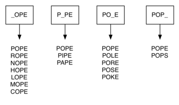
We can do much better by using the following approach. Suppose that we have a huge number of buckets, each of them with a four-letter word on the outside, except that one of the letters in the label has been replaced by an underscore. For example, consider the image below, we might have a bucket labeled “pop_.” As we process each word in our list we compare the word with each bucket, using the ‘_’ as a wildcard, so both “pope” and “pops” would match “pop_.” Every time we find a matching bucket, we put our word in that bucket. Once we have all the words in the appropriate buckets we know that all the words in the bucket must be connected.

wordbuckets

In java, this can be implemented using a Map as the obvious solution.. see the snippet below


for (String word : words) {
 for (int wordIndex = 0; wordIndex < word.length(); wordIndex++) {
   String keyWord = word.substring(0, wordIndex)+"_"+word.substring(wordIndex+1,word.length());
   if(!wordMap.containsKey(keyWord)){
    wordMap.put(keyWord, new ArrayList<String>());
   }
   wordMap.get(keyWord).add(word);
 }
}

Once we have the ‘well crafted’ map ready, it is easy to write this into a neo4j database.

  • For every word, a separate node is introduced
  • For every word under the same bucket, a relationship is made

Note : Neo4j don’t support the use of non-directional relationships. So, we go ahead and create a directional relationship and ignore the direction when we traverse the graph.

To write to the graph easily, a wrapper like the one shown below can be used,

public class WordGraph {

Map<String, Node> nodeMap;
GraphDatabaseService graphDb;

public WordGraph(){
  graphDb = NeoDatabaseHandler.getGraphDatabase();
  nodeMap = new HashMap<String, Node>();
}

private Node getNode(String word){
  if(!nodeMap.containsKey(word)){
   Node node = graphDb.createNode(NeoHelper.WordLabel.WORD);
   node.setProperty("word", word);
   nodeMap.put(word, node);
  }
  return nodeMap.get(word);
}

public void addEdge(String parentWord, String childWord){
  Node parentNode = getNode(parentWord);
  Node childNode = getNode(childWord);
  parentNode.createRelationshipTo(childNode, NeoHelper.RelationshipTypes.MOVE);
}
}

Whenever we need an edge created, we just call the method, addEdge and it will take care of the rest.

So, we iterate over the buckets and write the words and their relationships to the graph,

for (List<String> mappedWordsParent : wordMap.values()) {
  for (String parentWord : mappedWordsParent) {
    for (String childWord : mappedWordsParent) {
      if(!childWord.equals(parentWord)){
        wordGraph.addEdge(parentWord, childWord);
      }
    }
  }
}

The graph created using a minimum set of words will look like the one below, (apologies for the clutter in the relationship names)

Untitled


Once, we have the graph ready, we can do a decent traversal to get the required path. Let us assume, we are trying to find a path from fool to sage

The graph algorithm we are going to use is called the “breadth first search” algorithm. Breadth first search (BFS) is one of the easiest algorithms for searching a graph.

From a very neat post that i came across

Given a graph G and a starting vertex s, a breadth first search proceeds by exploring edges in the graph to find all the vertices in G for which there is a path from s. The remarkable thing about a breadth first search is that it finds all the vertices that are a distance k from s before it finds any vertices that are a distance k+1. One good way to visualize what the breadth first search algorithm does is to imagine that it is building a tree, one level of the tree at a time. A breadth first search adds all children of the starting vertex before it begins to discover any of the grandchildren.

Implementing this on our own, let us save that for another day. Neo4j provides a neat Traversal Framework.

Lets have a look at the code,

graphDb
.traversalDescription().breadthFirst()
                       .relationships(NeoHelper.RelationshipTypes.MOVE)
                       .evaluator(Evaluators.includeWhereEndNodeIs(endNode))
                       .traverse(startNode)

It’s pretty straight forward. We traverse through relationships named Move ( which is the only relationship we have in the Graph ). We use an Evaluator, which decides what to be returned as the output of a traversal, and in this case, we pass the node corresponds to the endword. So, whenever the traversal reaches the endword ( in this case sage), it returns the corresponding path. The complete code can be found in github.

Once, we have the path, printing it to standard out yields,

fool
pool
poll
pall
pale
sale
sage

Which is pretty much what we expected. You could try this out own your own as the entire project is available on github.

Much content has been adopted from this book, which is the ONE place you can start to understand data structures in python.


Adding DOM like features to Neo4j xml graph

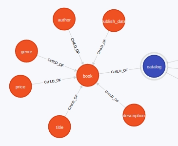
This is an extension to my previous post on how to convert an xml format data to a neo4j graph. For instance, see the graph generated an xml file in the following format

<?xml version="1.0"?>
<catalog>
<book id="bk101">
<author>Gambardella, Matthew</author>
<title>XML Developer's Guide</title>
<genre>Computer</genre>
<price>44.95</price>
<publish_date>2000-10-01</publish_date>
<description>An in-depth look at creating applications
with XML.</description>
</book>
.
.
.
</catalog>

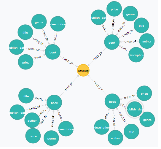
And the neo4j graph visualization below..

Catlog-xml

There are 4 <book> nodes under <catlog> and for each book, the associated metadata. Altogether it’s a pretty standard xml.

Most of our xml operations involve traversing the xml. JAXP is bread and butter for any developer working with xml in Java. I have done my bit of xml parsing and the interface provided is so wonderful (and resource intensive because of the DOM).

Similar flexibility is possible for the xmlGraph too..

I have tried to implemented the following methods..

  • getTags – Fetches the element objects for the specified xml tag
  • getParent – Fetches the parent element object
  • getChildren – Fetches the child element object
  • getSiblings – Fetches the siblings of the element

The implementation of the methods are in a separate service Facade..

public interface XmlTreeService {
  public List<XmlElement> getTags(String tagName);
  public List<XmlElement> getChildren(XmlElement parent);
  public XmlElement getParent(XmlElement child);
  public List<XmlElement> getSiblings(XmlElement element);
}

Implementation Details

Fetching the list of Tags, (the getTags method)

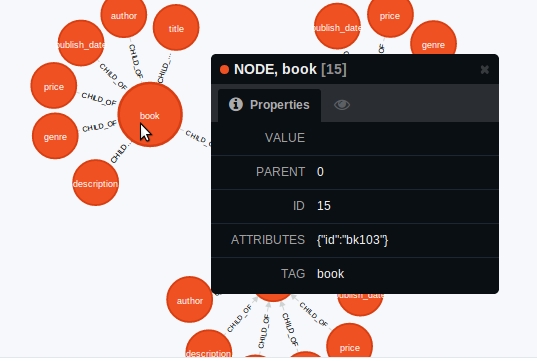
The best solution was to use the GlobalGraphOperations interface. As discussed before, while saving the xml as a graph, each node has it’s tag name as a label. For instance, the node representing a book node will have the label, ‘book‘ associated with it.

node-label-cropped


It can be seen the TAG property ‘book‘ is also a label.

This means fetching all Tags of a specified name resolves to fetching all nodes with a specific label, which is easy using GlobalGraphOperations

GlobalGraphOperations globalGraph = getGlobalGraphOperations();
Label label = DynamicLabel.label(tagName);
ResourceIterable<Node> nodes;
try (Transaction tx = graphDb.beginTx()) {
 nodes = globalGraph.getAllNodesWithLabel(label);
 for (Node node : nodes) {
   XmlElement element = getXmlElement(node);
   elements.add(element);
}
 tx.success();
} catch (IOException e) {
 LOGGER.severe(e.getMessage());
 e.printStackTrace();
}


Fetching the parent and children

In the graph we created, between a child tag and the parent tag in the xml, there exists a relationship, CHILD_OF from the child to the parent

child-of-crop

Implies finding the lineage is about finding the relationship of the node and fetching the element. For instance, see how the children nodes are fetched,


public List getChildren(XmlElement parent) {
 GraphDatabaseService graphDb = Neo4jDatabaseHandler.getGraphDatabase();
 List childElementList = new ArrayList<>();
 try(Transaction tx = graphDb.beginTx()) {
  Node node = graphDb.getNodeById(parent.getId());
  Iterable childRelations = node.getRelationships(Direction.INCOMING);
  Iterator relationshipIterator = childRelations.iterator();
  while(relationshipIterator.hasNext()) {
    Relationship relationship = relationshipIterator.next();
    Node childNode = relationship.getStartNode();
    XmlElement childElement = getXmlElement(childNode);
    childElementList.add(childElement);
  }
} catch (IOException e) {
// TODO Auto-generated catch block
 e.printStackTrace();
}

The process can be outlined as

  1. Fetch the node from GraphDatabaseService using the id which is stored in the XmlElement Object.
  2. Fetch the outgoing relationships which are INCOMING to the parent node.
  3. Iterate through the relationships and fetch the starting nodes.

The same method can be used to identify the parent node too..

Fetching Sibling Nodes

To fetch the sibling nodes, first fetch the parent node and then get the children. Also remove the node in question. Finding siblings is quite elementary.

You can always find the complete source code in github.

Summary

To roll all balls at once, let’s try to do a small test,

GraphDatabaseService graphDb = Neo4jDatabaseHandler.getGraphDatabase();
XmlTreeServiceGraph treeServiceGraph = new XmlTreeServiceGraph(graphDb);
System.out.println("-----Test for DOM like methods on XmlGraph----\n");
List<XmlElement> groupElements = treeServiceGraph.getTags("book");
System.out.println("Fetching all Book Nodes...");
for (XmlElement xmlElement : groupElements) {
  System.out.println(xmlElement.getAtrributeString());
}
XmlElement firstElement = groupElements.get(0);
System.out.println("\nFetching children of the first Book Node : " + firstElement.getAtrributeString() + "...");
List<XmlElement> childrenElements = treeServiceGraph.getChildren(firstElement);
for (XmlElement xmlElement : childrenElements) {
  System.out.println(xmlElement.getTagName()+ " : " + xmlElement.getTagValue());
}
XmlElement child = childrenElements.get(0);
System.out.println("\nFetching parent of the first child element : "+child.getTagName()+" : "+child.getTagValue() + "...");
XmlElement parentElement = treeServiceGraph.getParent(child);
System.out.println(parentElement.getTagName() + " : " + parentElement.getAtrributeString());
System.out.println("\nFetching siblings of the first Book Node : " + firstElement.getAttributes());
List<XmlElement> elementSibling = treeServiceGraph.getSiblings(firstElement);
for (XmlElement xmlElement : elementSibling) {
  System.out.println(xmlElement.getTagName() + " : " + xmlElement.getAtrributeString());
}


P.S : I know the test code is crappy, but for a demo test, this will do.. 🙂

So, it’s quite straightforward, I am doing the following steps

  1. Fetch all ‘book’ nodes in the xml, and print them
  2. Fetch all the children of the first ‘book’ node, and print them
  3. Fetch the parent of the first child from step #2, which should give us our first book node, and print them
  4. Fetch the siblings of the first node, and print them

Let’s see how the output looks like,

-----Test for DOM like methods on XmlGraph----

Fetching all Book Nodes...
{"id":"bk101"}
{"id":"bk102"}
{"id":"bk103"}
{"id":"bk104"}

Fetching children of the first Book Node : {"id":"bk101"}...
description : An in-depth look at creating applications with XML.
publish_date : 2000-10-01
price : 44.95
genre : Computer
title : XML Developer's Guide
author : Gambardella, Matthew

Fetching parent of the first child element : description : An in-depth look at creating applications with XML....
book : {"id":"bk101"}

Fetching siblings of the first Book Node : {id=bk101}
book : {"id":"bk104"}
book : {"id":"bk103"}
book : {"id":"bk102"}

It looks good, and everything as expected… 🙂

The Buendia Family Tree as a Neo4j graph – Tribute to Gabo

One of the most significant and prominent authors passed away last fortnight – Gabriel Garcia Marquez. I read One Hundred Years of Solitude during my senior college years. Magical Realism has long been associated with the vernacular literature in my home state.

gabriel-garcia-marquez

The Buendia family in One Hundred Years of Solitude is another epic on it’s own. See a very nice graphic family tree below.

100_years_of_solitude_family_t_by_clothos

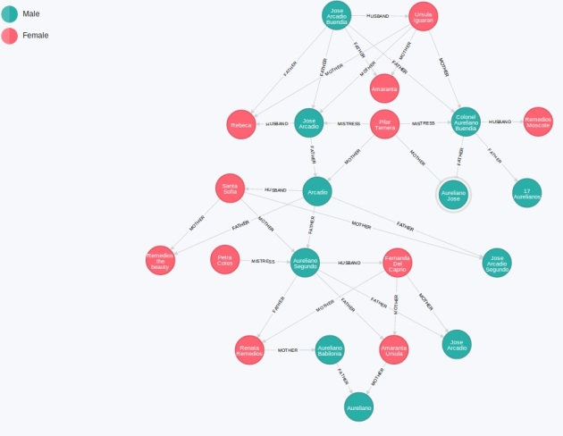
I always wanted to visualize a family tree using a graph, and the Buendias of Macondo seemed so perfect. My other choice was the political families of India, which is pretttyyy vaasttt..

The visualization is pretty straightforward, two types of nodes

  • Male
  • Female

And 4 simple relationships

  • HUSBAND
  • FATHER
  • MOTHER
  • MISTRESS (Sorry, could not find an euphemism for that)

final-buendia-crop

Apologies if it is too cluttered, but you could play around with the graphgist